This time of year, M57 (the ring nebula) is advantageously located in our night sky, so this is a good opportunity to discuss astrophotography.

The basic problem to be solved is that the objects are of very low intensity and are moving. Here’s a sample image:

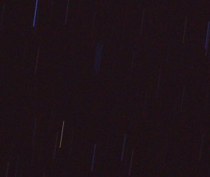
This is a 20-second exposure using our 800mm f/5.6 lens, ISO 2000. Because we know how fast the stars are (apparently) moving- 360 degrees in 24 hours- we can calculate how long the shutter could be open before this motion blur occurs. For this lens and camera (pixel size = 6 microns, but there is a Bayer filter present), the maximum shutter speed is about 1/4 second: within 1/4 second, the stars move less than a pixel. That’s suboptimal, to say the least. We could try to improve things by using a faster lens and higher sensor gain, but our setup is already close to the limit of what is commercially available.

The solution is to use a ‘tracking mount‘. There are lots of different designs, ours is a ‘German equatorial mount‘. The basic procedure is very simple- align the polar axis of the mount to the North star and turn on the motors. When aligned, The two motors correspond to declination (latitude) and right ascension (longitude). Then, the mount essentially ‘unwraps’ the Earth’s rotation, ensuring the telescope remains pointed at the same part of the night sky. This is also a 20-second exposure, but taken with the tracking mount aligned:

much better! The final step is to take a lot of these images and average them all together (‘image stacking’).

Naturally, life is not as simple as that. Most images look like this:

What’s the deal? There are lots of reasons why this image still has motion blur: vibrations, polar misalignment, gear error, etc., and it’s illuminating to calculate acceptable limits. First, let’s dispense with the pixel size issue- the sensor dimensions result in a single ‘pixel’ as being 6 microns on a side. However, in order to generate color images, a Bayer filter is placed over the pixel array, so that neighboring pixels are assigned different colors (and detect slightly different parts of the object). A detailed analysis is highly complicated- 3 independent non-commensurate samplings of the image plane- but if our image does not have features smaller than say, 12 microns (corresponding to a 2×2 pixel array), software interpolation that generates a color pixel using the neighboring elements will likely give an accurate result, and we can pretend that our sensor has 6-micron color pixels.

And in fact, examining our ‘best’ single image, stars are imaged as bright blobs of radius 3 pixels (and brighter stars appear as even bigger blobs).

Ok, so how much can the sensor move without causing motion blur? The stringent limit is that the sensor (or the image projected onto the sensor) must move less than 0.5 pixel (3 microns) during an exposure. If the lever arm of the lens is 0.5m, the allowed angular displacement is 1.2 arcsec. In terms of vibrations, this is a very stringent requirement! Similarly, we can calculate the maximum allowed polar misalignment: if the telescope pointing is allowed to drift no more than 0.5 pixel during an exposure, since each pixel subtends 1 arcsec (for diffraction-limited performance using this lens), the allowed misalignment is about 6 arcmin (http://canburytech.net/DriftAlign/DriftAlign_1.html is a good reference).

Speaking of diffraction-limited, what is the limit of our system? Each star should be imaged as a single pixel! Clearly, there is image degredation not just from movement, but from *seeing*- clear air turbulence appears as blur in long time exposures. How much degredation? Our “best” images correspond to using a lens at f/30, or an entrance pupil diameter of 27mm (instead of f/5.6, 140 mm entrance pupil diameter). The seeing conditions in Cleveland are *awful*!

So why do astrophotography? Our images are not meant to compete with ‘professional’ telescope images. It’s also a nice experience to learn about the night sky and work on our imaging technique. Here’s the result of stacking enough ‘best’ 20-second exposure images to produce a single 29 minute long exposure:

Not bad! And we can continue to improve the image- either by ‘dithering’ the individual frames to allow sub-pixel features to emerge:

or by deconvolving the final image, using a 3-pixel radius Gaussian blob as the point-spread function:

The image improvements may not appear that significant, but as always, the rule of post-processing is *subtle* improvements- no artifacts must be introduced.

The American Institute of Physics journal “Physics of Fluids” sponsors a ‘gallery of fluid motion’ every year (http://pof.aip.org/gallery_of_fluid_motion) and without fail, the selected images are breathtakingly amazing. Our images don’t make the cut.

Fortunately, we can display our own gallery of fluid motion right here. The following images were all taken at Cape Hattaras, North Carolina, part of the Outer Banks, infamous for the number of shipwrecks caused by sandbars located all along the coast.

Let’s discuss waves- specifically, ocean waves that break onto the beach. This is a ubiquitious phenomenon (especially if you include lakes, not to mention waves formed by sloshing around a tank), and yet the mathematics behind these structures is hideously complex.

It’s not clear why, but fluid mechanics (and its parent discipline, continuum mechanics) is essentially absent from the Physics curriculum. The mathematics are well established- classical field theory, differential geometry , etc- and the physical concepts are well posed (homogeneous/multiphase systems, thermodynamics, conservation laws, etc.) but nearly all the interesting work has been left to mathematicians and engineers (who have produced a stunningly beautiful body of knowledge). Stoker’s “Water Waves” is an especially good reference.

The problem of waves falls under the general problem of ‘interfacial phenomena’ and ‘free surface flows’, which are the red-headed stepchildren of continuum mechanics- the fluid-fluid boundary is no longer specified but is free to deform, so the interface shape is now part of the overall problem to be solved. Also, the no-slip boundary condition no longer holds. And as we will see, even the hypercomplicated problem of a free surface dividing two homogeneous Newtonian fluids is simple compared to the typical complexities of real ocean waves.

For now, consider the interface between water and air as a two-dimensional surface, referred to as a Gibbs dividing surface, possessing physical properties independent of either bulk material. The curvature of the surface is proportional to the pressure jump across the surface, for example. Also, when we say ‘fluid’, we generally mean the seawater, as opposed to the atmosphere.

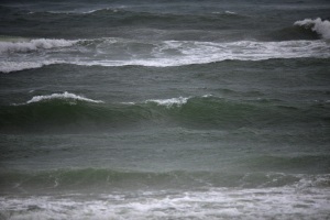
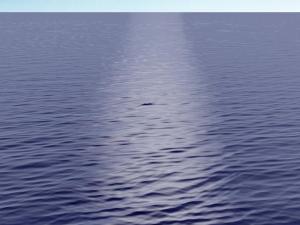
Let’s start with an image of the ocean surface far from the shore:

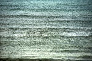
This surface is dominated by long-wavelength waves (long waves) parallel to the beach covered by fairly uniform short-wavelength ripples. The dynamics of this image are fairly well understood- the wavespeed, dispersion relations, the overall velocity field within the bulk fluids, etc. – because the height of the waves is much smaller than the depth of the fluid, and the depth of the fluid is constant over many wave periods. Perturbative approaches are well suited to this problem and have produced useful results. For example, the speed of the wave is sqrt(gh), where h is the height of a wave and ‘g’ is 9.8 m/s^2.

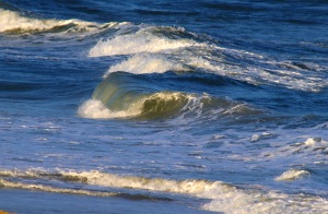
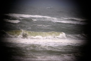
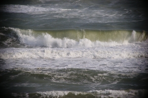
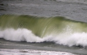
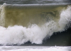
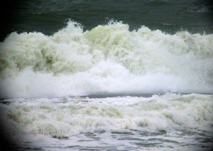
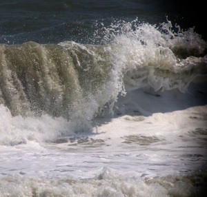
However, as the waves approach the shore, the fluid depth changes rapidly, resulting in ocean fluid ‘piling up’ behind the wavefront and eventually breaking over the top, which is more visually appealing:

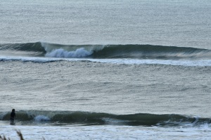
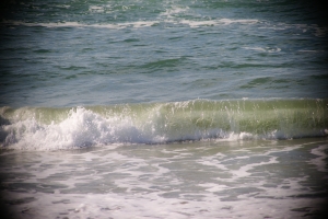
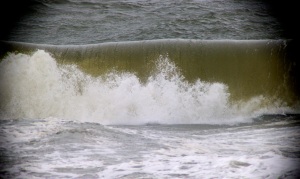
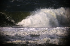
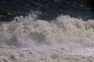
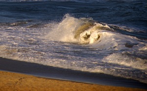
The upper image is useful to get a sense of scale- the front wave is about 3 feet high, while the rear wave is closer to 6 feet. For now, we will only discuss these ‘medium’ waves- of height 3-6 feet. The lower image is of a 3-foot wave, and displays a very uniform ‘phenotype’- very regular height and cylindrical profile, justifying 2-D treatments of the problem. Let’s look at the waves from a more oblique angle:

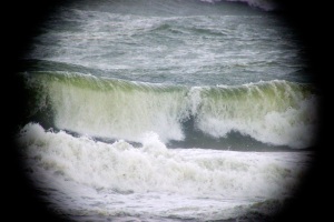
In these images, it’s possible to see what looks like ‘viscous fingering’- the wavefront divides into multiple ‘fingers’, which break independently.

Now let’s focus on the crest of a wave- it turns out that the height of the crest is proportional to the depth of the water- the larger wave, further out, is in deeper water. The wave crests (‘breaks’) when the slope becomes infinite (vertical). Short waves break sooner than long waves, and breaking occurs faster as the uniform ‘background’ fluid velocity decreases- when a wave breaks and retreats (negative velocity), the following wave breaks much sooner. Where the wave crests, and how high the wave is at cresting, tells us information about the spatial variations in ocean depth.

A note about how these images (and the remainder) were taken. Primarily, a 400/2.8 (or 800/5.6 using the 2x tele) lens was used, and the optimal lighting conditions are usual for capturing fluid motion- lots of light (direct sunlight), ‘harsh lighting’ (lots of contrast), and fast shutter speeds- 1/1000s or faster. Consequently, the lens was used at full aperture, resulting is a narrow depth of field- it was tricky to get the wave in focus, but when it is in focus , each droplet of water can produce a little flash of light like a star. It’s worth looking at these images full-scale, there is a lot of detail.

We should now pause and ask about the origin of the fluid velocity- the motive force, so to speak. The origin of tidal flow is due to the moon, but what is the origin of ocean waves?

The source of waves is wind: air flowing over the ocean surface. No air, no waves. The waves propagating to shore were produced by wind far offshore- thus the character of waves tells us about the weather conditions far offshore- stormy, calm, etc. The direction of airflow is not really correlated with ocean currents, thus another complication is that the problem is intrinsically 3-dimensional. Yep, no interesting physics here…

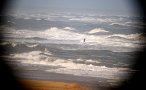
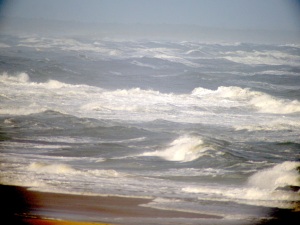
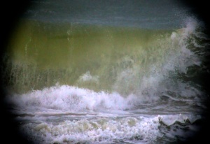
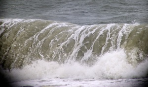
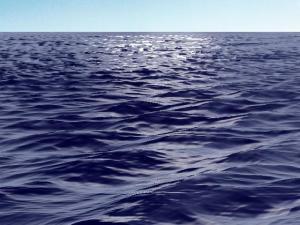
So, let’s add wind: it should be clear that some images were taken when the offshore weather was relatively calm, while others were taken when a storm was present- the waves are bigger and more closely spaced. Here is what happens when an on-shore 30 mph wind is added, blowing from the shore into the water, as a storm came onshore:

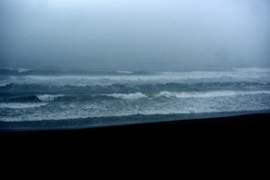
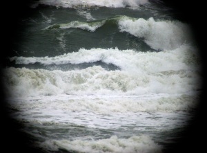
The waves appear much different- less cresting, flatter waves.

Upon closer examination of the images, additional features appear- the waveheight varies along the crest, for example, and in addition to the long-wavelength variation of wave height, there is a short-wavelength feature as well, and the top of the cresting wave takes on a ‘glassy’ appearance. As the wave crests, the crests merge at semi-regular intervals to form a ‘seam’.

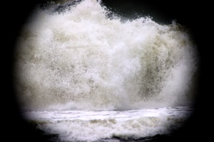
What about larger waves, 10-15 feet in height. Do they appear similar or different?

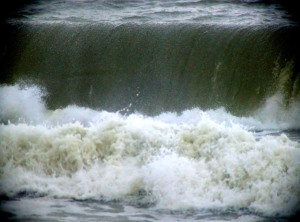
What about the splash as the wave falls back onto the water?

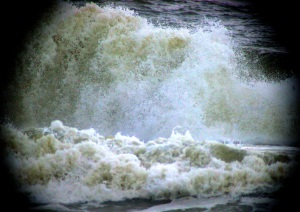
What if we allow the mechanical properties of one of the fluids to change- foam formed by the waves can build up and mix with the fluid, changing the ocean fluid from a simple Newtonian fluid into a visco-elastic fluid- note the thicker ‘ropey’ structure.

Clearly, ocean waves display a complex behavior that is difficult to model. And we haven’t yet discussed the sand under the water- it’s a granular material that can flow, and in fact forms structures that look like dunes, in an orientation parallel to the waves. So we have, in general, a time-dependent 3-D mechanics problem involving a homogenous fluid (air), an inhomogenous fluid (the ocean water/foam) and a granular material (sand). If we wanted, we could add thermodynamics to the problem- to model solar heating, for example.

Let’s see how the computer graphics special effects folks do:(from http://hal.inria.fr/UNIV-GRENOBLE1/inria-00537490)

Not bad for calm water- but recall, that first image up top is very amenable to modeling. Here’s a still from “Surf’s Up”: (http://news.cnet.com/8301-13772_3-9862945-52.html)

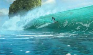
Also not bad (Sony *did* get an Oscar nomination for this, after all)- but it’s not clear how much of the animation was based on physics and how much was smart illustration (http://library.imageworks.com/)

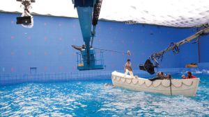
Here it’s clear that the model can’t compare to reality- the wave surfaces are *way* too smooth. In order to get realistic waves, Ang Lee used a giant tank for his movie, “Life of Pi”:

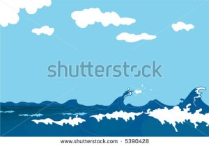
Illustrators can do a better job of capturing the dynamics, but omit a lot of detail:

That said, it’s important to remember that we can simplify the problem and extract out useful information- the 2D approximation for long waves is one simplification. Modeling ocean waves, while useful for various industries, can be applied to other problems as well- for example, airflow within the lung. Within the airway there is a homogeneous fluid (air), viscoelastic fluid (mucus/airway surface liquid), and a deformable soft matter layer (epithelial tissue). The air can be seeded with particulate matter (airbourne contamination), and we can model where those particles are likely to accumulate in the airway. We can also model the effects of adding a surfactant, often used as a medical intervention for premature newborns who don’t have a well-developed lung.